Tutorial 2 - Handling discontinuities
Often, real-world integration problems in engineering have discontinuities. That means that the physics cannot be described adequately by a single set of equations.
Fortunately, npsolve provides a soft_functions module to make it easy to handle discontinuities, by preventing them entirely. These functions work by providing a differential that changes smoothly over a very, very small time, distance, or whatever value it’s applied to. Variable time step solvers, such many in in scipy.integrate, handle these very small but smooth transitions easily. The approximation of these functions inevitably introduces small errors, but for many real-world problems these errors are negligible. It’s far more important to get a 99.999% accurate result than none at all.
We’ll illustrate the use of two soft_functions to model a bouncing ball. It’s going to start rolling along a ledge, before falling off onto a surface that it bounces on. Let’s start with some setup:
import numpy as np
from scipy.integrate import odeint
import matplotlib.pyplot as plt

import npsolve
from npsolve.soft_functions import negdiff, below

G = -9.80665
Y_SURFACE = 1.5
X_LEDGE = 2.0
Y_LEDGE = 5.0
POS = "position"
VEL = "velocity"
Both POS and VEL will be np.arrays of length 2, representing values in the x and y axes.
The Ball class
Now we’ll start writing our Ball class. We’ll give it some mass and some parameters to control how it bounces. We’ll create the bouncing by a combination of spring-like behaviour and velocity-dependent damping. Here’s the constructor:
class Ball:
    def __init__(self, mass=1.0, k_bounce=1e7, c_bounce=3e3):
        self.mass = mass
        self.k_bounce = k_bounce
        self.c_bounce = c_bounce
Let’s create a method in the Ball class to calculate the force of gravity on the ball.
class Ball():
    # ...

    def F_gravity(self):
        """ Force of gravity """
        return np.array([0, self.mass * G])
Pretty simple so far. Now let’s make our ledge react the force of gravity until the ball reaches the edge of the ledge with another method:
class Ball():
    # ...

    def F_ledge(self, state):
        x_pos = state[POS][0]
        return -self.F_gravity() * below(x_pos, limit=X_LEDGE)
Here, we’re using the below soft function. It’s 1 below a limit (here X_LEDGE) and 0 above it, with a very small but smooth transition around the limit. So, this force will only apply until the ball reaches the edge of the ledge. We do this so the differentials are continuously smooth, so the scipy integrator won’t have any trouble with discontinuities.
Now, let’s make the method to generate a bouncing force when it hits the surface. This one is a bit more complex:
class Ball():
    # ...

    def F_bounce(self, state):
        """Force bouncing on the surface"""
        y_pos = state[POS][1]
        y_vel = state[VEL][1]
        F_spring = -self.k_bounce * negdiff(y_pos, limit=Y_SURFACE)
        c_damping = -self.c_bounce * below(y_pos, Y_SURFACE)
        F_damping = c_damping * negdiff(y_vel, limit=0)
        return np.array([0, F_spring + F_damping])
We’re using the negdiff soft function here. It gives the difference between a value and some limit when the value is below the limit and 0 when it’s above. Again, it’s a smooth function with a very small transition region around the limit. We apply that to the spring force so it only provides that force when the ball is (slightly) below the surface.
For the damping, we’ve used the below function to set up a damping coefficient, c_damping, that will only apply when the ball is (slightly) below the surface. We also want the damping force to only push the ball - we don’t want it to ‘pull’ the ball like a sticky surface might. So, we’ve used the negdiff function on the velocity. When the velocity is positive, the negdiff function goes to 0 so the damping force will be 0 too. We add the two forces to return a bounce force.
Now we can set up the step method that gets called by the integrator.
class Ball():
    # ...

    def step(self, state, t, log):
        """Called by the solver at each time step"""
        F_net = self.F_gravity() + self.F_ledge(state) + self.F_bounce(state)
        acceleration = F_net / self.mass
        derivatives = {POS: state[VEL], VEL: acceleration}
        return derivatives
This just sums the forces, calculates the acceleration by applying elementary physics, then returns the acceleration.
The System
Now let’s set up the System:
def get_system():
    ball = Ball()
    system = npsolve.System()
    system.add_component(ball, "ball", "step")
    return system
This system configuration is extremely simple, with only one component with one final call to get the derivatives.
Running
We’ll use npsolve.integrate to solve the solution.
def run(t_end=3.0, n=100001):
    system = get_system()
    inits = {
        POS: np.array([0.0, Y_LEDGE]),
        VEL: np.array([5.0, 0.0]),
    }
    system.setup(inits)
    dct = npsolve.integrate(system, t_end=t_end, framerate=(n - 1) / t_end)
    return dct
We’ll also add a function to plot results.
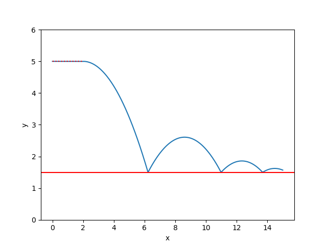
def plot(dct):
    plt.figure()
    plt.plot(dct[POS][:, 0], dct[POS][:, 1], label="position")
    plt.axhline(Y_SURFACE, c="r")
    plt.plot([0, X_LEDGE], [Y_LEDGE, Y_LEDGE], "r:")
    plt.ylim(0, 6)
    plt.xlabel("x")
    plt.ylabel("y")
    plt.show()
Results
Let’s add function to run it and plot results.
def execute():
    dct = run()
    plot(dct)


if __name__ == "__main__":
    execute()
We’ve made a bouncing ball!
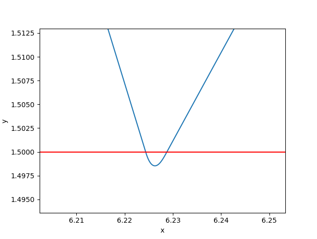
If we zoom way in on the bounce, you can see it’s actually smooth. This is because of the soft function we used.