Tutorial 4 - Sharing values between objects

In more complex models, values often need to be shared between different Partial instances. Sometimes, those values are state variables that are declared with the add_var method. In that case, any Partial connected to the Solver will get access to them through their state dictionary (i.e. self.state[<variable name>]). But some shared values are not state variables. How do we handle that?

We use the fastwire package. It provides a convenient, event-like way to share variables. This tutorial will give an example. We’re going to simulate the dynamics of a frictionless slider moving in the x axis with a pendulum attached that is free to move in the x and y axes. We’ll add a sinusoidal force to the slider to excite the system dynamics.

First, a little setup:

import numpy as np
import matplotlib.pyplot as plt
import npsolve
from tutorial_2 import run

G = np.array([0, -9.80665])

Here, we’ve made G a 2D vector to represent gravity.

Now we’ll get a wire box. A wire box is a collection of wires that we’ll use to pass values. Here’s how we do that:

import fastwire as fw
wire_box = fw.get_wire_box('demo')

You can use wire_box = fw.get_wire_box(‘demo’) in any code module and it’ll get the same wire box, so you don’t have to import that object into other modules.

Now let’s start making the Slider.

class Slider(npsolve.Partial, fw.Wired):
    def __init__(self, freq=1.0, mass=1.0):
        super().__init__() # Don't forget to call this!
        self.freq = freq
        self.mass = mass
        self.add_var('s_pos', init=np.zeros(2))
        self.add_var('s_vel', init=np.zeros(2))

Importantly, we’re inheriting the fw.Wired class. That lets us use fastwire decorators. We’re also making the Slider fully 2D, even though at this stage we only want it to move in x.

We’re doing to connect the Pendulum to the Slider, and the Pendulum will need to know where the Slider is so it can pivot about the right point. Here’s how we make the pivot location and velocity available to the Pendulum:

class Slider(npsolve.Partial, fw.Wired):
    # ...

    @wire_box.supply('pivot')
    def pivot(self, t):
        """ The location of the pivot that connects to the pendulum """
        return self.state['s_pos'], self.state['s_vel']

We decorate the method with @wire_box.supply(‘pivot’) because we’ve called our wire box wire_box. This tells fastwire that this method supplies the values referred to by the wire called ‘pivot’. We’ll pass in the current time, t, although we don’t need it yet.

Let’s set up a method to create the excitation force:

class Slider(npsolve.Partial, fw.Wired):
    # ...

    def F_sinusoid(self, t):
        """ The force to make the system do something """
        return 10 * np.cos(2 * np.pi * (self.freq * t))

Now we can write our step method to return the state derivatives by doing some basic physics.

class Slider(npsolve.Partial, fw.Wired):
    # ...

    def step(self, state_dct, t, *args):
        """ Called by the solver at each time step  """
        F_pivot = -wire_box['F_pivot'].fetch(t)
        F_pivot_x = F_pivot[0]
        F_sinusoid_x = self.F_sinusoid(t)
        F_net_x = F_pivot_x + F_sinusoid_x
        acc = np.array([F_net_x / self.mass, 0])
        derivatives = {'s_pos': state_dct['s_vel'],
                       's_vel': acc}
        return derivatives

Notice here we’re going to pull in a force, F_pivot, which is going to be calculated by the Pendulum class. We just have to use the fetch method on the right wire, which here we’ve called F_pivot. For this example, we’ll also pass in the current time ‘t’ to the method that will supply that force (we haven’t written that method yet). We’re flipping the sign because the slider will see the reaction force.

Now, let’s make the Pendulum class.

class Pendulum(npsolve.Partial, fw.Wired):
    def __init__(self, mass=1.0, k=1e6, c=1e4, l=1.0):
        super().__init__() # Don't forget to call this!
        self.mass = mass
        self.k = k
        self.c = c
        self.l = l
        self.add_var('p_pos', init=np.array([0, -self.l]))
        self.add_var('p_vel', init=np.array([0, 0]))

Again, we’re inheriting fw.Wired. This class has some stiffness (k) and damping c parameters, along with mass (mass) and length (l). It needs to calculate the force that arises because of it’s connection to the Slider. We’re going to model a very stiff, damped connection between the pivot on the Slider and the position of the Pendulum.

class Pendulum(npsolve.Partial, fw.Wired):
    # ...

    @wire_box.supply('F_pivot')
    @npsolve.mono_cached()
    def F_pivot(self, t):
        """ Work out the force on the pendulum mass """
        pivot_pos, pivot_vel = wire_box['pivot'].fetch(t)
        rel_pos = pivot_pos - self.state['p_pos']
        rel_vel = pivot_vel - self.state['p_vel']
        dist = np.linalg.norm(rel_pos)
        unit_vec = rel_pos / dist
        F_spring = self.k * (dist - self.l) * unit_vec
        rel_vel_in_line = np.dot(rel_vel, unit_vec)
        F_damping = self.c * rel_vel_in_line * unit_vec
        return F_spring + F_damping

We’re again using the @wire_box decorator so that this method will supply the F_pivot wire. The return value, the force at the pivot, will be used by both the Slider (via the F_pivot wire) and the Pendulum (directly). We can’t assume which object will call the F_pivot method first, but we don’t want to have it calculate the result twice. (This is a simple example, but in computationally intensive calculations, reducing calculations can be important.) So, we use the @npsolve.mono_cached() decorator here as well. This caches the result for the current timestep. Subsequent calls simply return that value. The mono_cached() doesn’t care about the value of arguments. If they might change for the same timestep, you can use the multi_cached() decorator instead.

Let’s add the force of gravity now:

class Pendulum(npsolve.Partial, fw.Wired):
    # ...

    def F_gravity(self):
        return self.mass * G

Finally, we’ll make the step method, doing some basic physics to calculate acceleration.

class Pendulum(npsolve.Partial, fw.Wired):
    # ...

    def step(self, state_dct, t, *args):
        ''' Called by the solver at each time step
        Calculate acceleration based on the
        '''
        F_net = self.F_pivot(t) + self.F_gravity()
        acceleration = F_net / self.mass
        derivatives = {'p_pos': state_dct['p_vel'],
                       'p_vel': acceleration}
        return derivatives

Before we run, let’s make some plot functions…

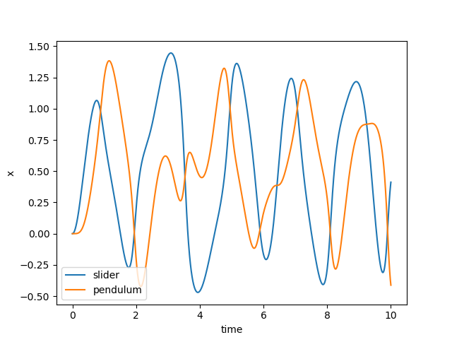
def plot_xs(dct):
    plt.plot(dct['time'], dct['s_pos'][:,0], label='slider')
    plt.plot(dct['time'], dct['p_pos'][:,0], label='pendulum')
    plt.xlabel('time')
    plt.ylabel('x')
    plt.legend(loc=3)


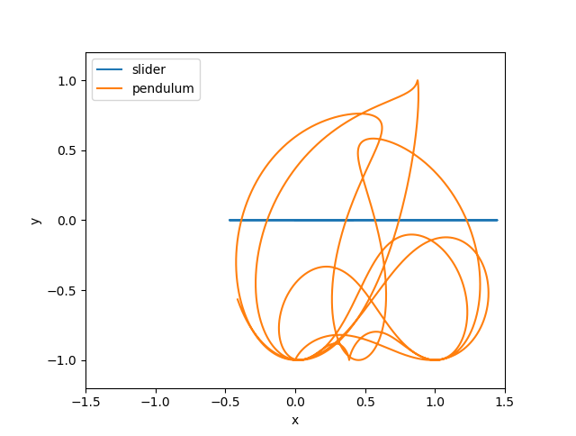
def plot_trajectories(dct):
    plt.plot(dct['s_pos'][:,0], dct['s_pos'][:,1], label='slider')
    plt.plot(dct['p_pos'][:,0], dct['p_pos'][:,1], label='pendulum')
    plt.xlabel('x')
    plt.ylabel('y')
    plt.xlim(-1.5, 1.5)
    plt.ylim(-1.2, 1.2)
    plt.gca().set_aspect('equal')
    plt.legend(loc=2)

Finally, we’ll make a little function to run the model and plot the results.

def execute(freq):
    partials = [Slider(freq=freq), Pendulum()]
    dct = run(partials, t_end=10.0, n=10001)
    plot_xs(dct)
    plot_trajectories(dct)

Let’s see what happens at 2 Hz:

execute(2.0)

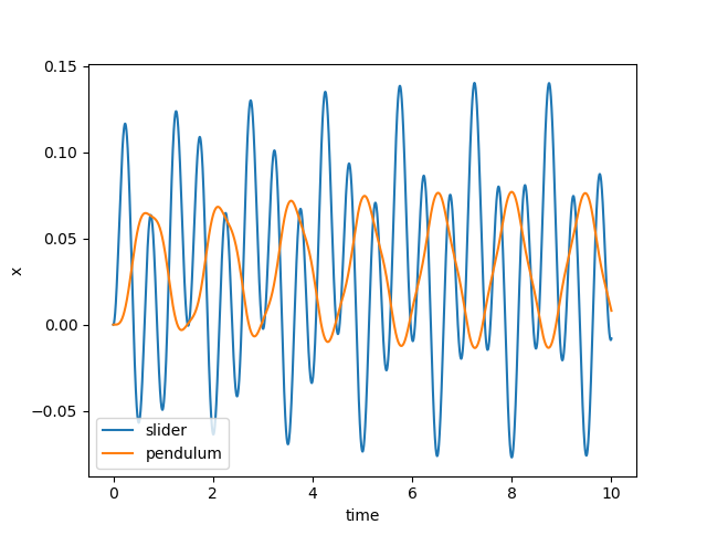
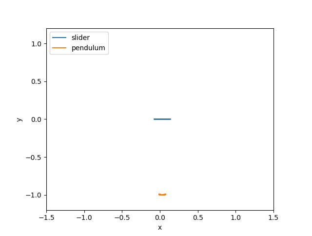
Nothing very interesting. Both objects just oscillate, as you might expect. Now let’s try at 1 Hz:

execute(1.0)

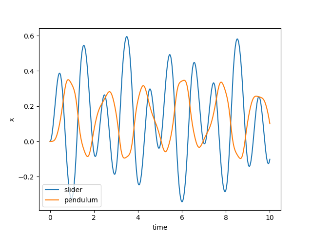
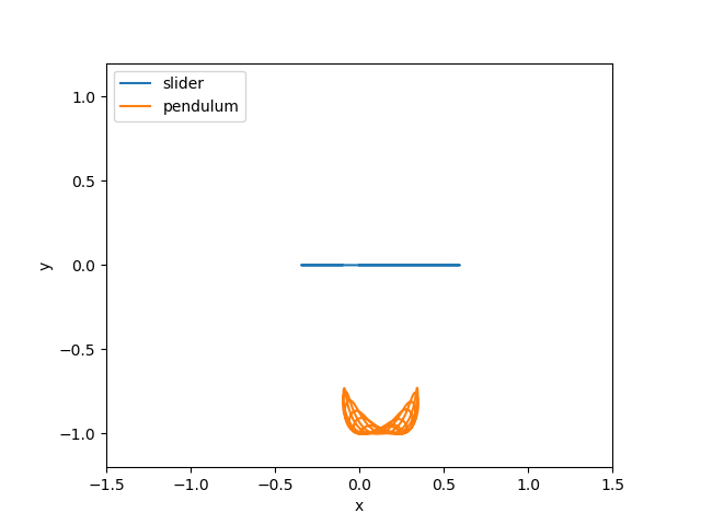
The Pendulum is wobbling around a bit more now. Let’s try at 0.5 Hz:

execute(1.0)

When we look a the trajectories, we see what’s really happening…

Remember that our pendulum isn’t quite a rigid body - we’ve approximated it as a very stiff, highly damped spring. We should check that the approximation is good by checking that the distance between the pivot and pendulum is very very close to 1.0. Let’s plot the distance:

def plot_distance_check(dct):
    diff = dct['p_pos'] - dct['s_pos']
    dist = np.linalg.norm(diff, axis=1)
    plt.plot(dct['time'], dist)
    plt.xlabel('time')
    plt.ylabel('length')

plot_distance_check(dct)

Our maximum length error is only 0.0001, compared to our pendulum length of 1.0, so we know the errors due to that approximation will be small.