Tutorial 5 - Using polymorphism

In Tutorial 4, we made a Pendulum move under a Slider. What if that pendulum moved under the Particle we made in Tutorial 3 instead? Let’s find out, to demonstrate how npsolve makes it easy to do so.

We’ll start by importing what we need:

import numpy as np
import matplotlib.pyplot as plt
from tutorial_2 import run as t2_run
from tutorial_3 import Particle
from tutorial_4 import Pendulum
import fastwire as fw
wire_box = fw.get_wire_box('demo')

We need to add a pivot method to the Particle, so we’ll subclass it like this.

class Particle2(Particle, fw.Wired):

    @wire_box.supply('pivot')
    def pivot(self, t):
        velocity = np.array([self.xts(t, der=1), self.yts(t, der=1)])
        return self.state['position'], velocity

That’s it - now this class will substitute for the old Slider class! We’re returning the position and velocity in the same format that the Pendulum expected from the Slider, and we’ve wired it to the same ‘pivot’ wire.

There’s one small glitch - initial conditions. In Tutorial 4, we conveniently set up the initial conditions right. How do we do that now? Here’s how:

def set_init_condition(particle, pendulum):
    init_particle_pos = particle.npsolve_vars['position']['init']
    init_pendulum_pos = init_particle_pos - np.array([0.0, 1.0])
    pendulum.set_init('p_pos', init_pendulum_pos)

When a class calls add_var, that information gets added to the npsolve_vars attribute. We’re taking that, subtracting our pendulum length from the height, and then calling the set_init method to set the initial position of the pendulum to that position. Easy.

Now we’ll make a function to run the new model.

def run(k=1e6, c=1e4):
    particle = Particle2()
    pendulum = Pendulum(k=k, c=c)
    set_init_condition(particle, pendulum)
    partials = [particle, pendulum]
    dct = t2_run(partials, t_end=1.0, n=10001)
    return dct

And a new plot function to see the results.

def plot_trajectories(dct):
    plt.plot(dct['position'][:,0], dct['position'][:,1], linewidth=1.0,
             label='particle')
    plt.plot(dct['p_pos'][:,0], dct['p_pos'][:,1],  linewidth=1.0,
             label='pendulum')
    plt.xlabel('x')
    plt.ylabel('y')
    plt.xlim(-2.5, 12.5)
    plt.ylim(-2.5, 12.5)
    plt.gca().set_aspect('equal')
    plt.legend(loc=2)

Let’s run it!

dct = run()
plot_trajectories(dct)

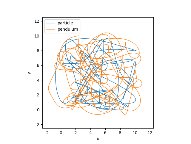
Our pendulum is now hurtling around with a particle!

Let’s check the pendulum length again to ensure it’s behaving as expected.

def plot_distance_check(dct):
    diff = dct['p_pos'] - dct['position']
    dist = np.linalg.norm(diff, axis=1)
    plt.plot(dct['time'], dist)
    plt.xlabel('time')
    plt.ylabel('length')

plot_distance_check(dct)

Here, our stiff spring and firm damping aren’t quite enough to handle the fast accelerations due to the particle motion. So, we’ll tweak our parameters and run again:

dct = run(k=1e9, c=1e7)
plot_trajectories(dct)
plot_distance_check(dct)

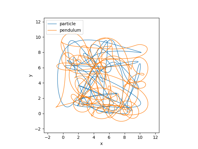
Our Pendulum trajectory is different.

Now, our distance check looks ok, so we can be more confident with this result - as crazy as it is!

Think about what this lets us do. We might write classes for a given situation. Then, say if we run an experiement and get some measured data, we can swap the relevant Partial for one that uses that Timeseries data. Or, perhaps we have a new idea to test - we can easily swap out that part of the model and compare it back to back with the first.

We can validate our classes against unittests, theory, and experimental data. Then, we can run new models that use them without changing anything within those classes. This can provide confidence that we haven’t made any mistakes within those classes in the new model.