Tutorial 1 - Basics

Let’s use npsolve to do some integration through time, like you would to solve an ODE. Instead of equations, though, we’re using class methods.

Imports

Let’s start with some imports we’ll need.

import numpy as np
import npsolve
import matplotlib.pyplot as plt

Setting up variable names

First, setup some variable names for the states that will be integrated. These may be floats or 1-dimensional np.ndarrays. Their names must be unique.

# Unique variable names
COMP1_POS = "position1"
COMP1_VEL = "velocity1"
COMP2_VALUE = "component2_value"
COMP2_FORCE = "comp2_force"

Component classes

Now, let’s set up some objects to do the calculations. We’ll give each component a step method, although we could use any name for the methods. The first three arguments passed to these methods will be, state, t, and log.

`state`: A dictionary of the current state for all parameters.
`t`: The time for the curren step.
`log`: Either None, or a dictionary. By setting key-value pairs in this

dictionary for each time step, additional non-state variables can be included in the results.

class Component1:
    def set_comp2_force(self, force):
        self._comp2_force = force

    def get_pos(self, state):
        return state[COMP1_POS]

    def step(self, state, t, log):
        """Called by the solver at each time step

        Calculate acceleration based on the net component2_value.
        """
        acceleration = self._comp2_force * 1.0
        derivatives = {
            "position1": state[COMP1_VEL],
            "velocity1": acceleration,
        }
        return derivatives


class Component2:
    def get_force(self, state):
        return 1.0 * state[COMP2_VALUE]

    def set_comp1_pos(self, pos):
        self._comp1_pos = pos

    def calculate(self, state, t):
        """Some arbitrary calculations based on current time t
        and the position at that time calculated in Component1.
        This returns a derivative for variable 'c'
        """
        dc = 1.0 * np.cos(2 * t) * self._comp1_pos
        derivatives = {COMP2_VALUE: dc}
        return derivatives

    def step(self, state, t, log):
        """Called by the solver at each time step"""
        return self.calculate(state, t)

Now, notice that Component1 needs a value called comp2_force, which Component2 should calculate. This needs to somehow be passed to Component1. Likewise, Component2 needs to be passed a position from Component1. How can we achieve this while still encapsulating the calculations that each component is responsible for with the component?

Managing interdependencies

It’s common to have interdependencies between components. To manage them, we’ll create another class to inject the interdependencies at the right time that we’ll call Assembly.

class Assembly:
    """Handle inter-dependencies."""

    def __init__(self, comp1, comp2):
        self.comp1 = comp1
        self.comp2 = comp2

    def precalcs(self, state, t, log):
        """Inject dependencies for later calculations in 'step' methods."""
        comp1 = self.comp1
        comp2 = self.comp2
        comp1_pos = comp1.get_pos(state)
        comp2_force = comp2.get_force(state)
        if log:
            # Log whatever we want here into a dictionary.
            log[COMP2_FORCE] = comp2_force
        comp1.set_comp2_force(comp2_force)
        comp2.set_comp1_pos(comp1_pos)

Let’s have a look at the precalcs method. It accepts state, t, and log, so it can be called during each time step. It gets values from each component and then injects them into the other one, so their step methods will have the right values.

Setting up the System

Now it’s time to link instances of all these components together for use during integration. For this, we use the npsolve.System object. Here, we’ll make a function to create instances of our components, create a System instance, and add the components to it.

def get_system():
    component1 = Component1()
    component2 = Component2()
    assembly = Assembly(component1, component2)
    system = npsolve.System()
    system.add_component(component1, "comp1", "step")
    system.add_component(component2, "comp2", "step")
    system.add_component(assembly, "assembly", None)
    system.set_stage_calls([("assembly", "precalcs")])
    return system

Let’s look at what’s going on. The first four lines are simply creating instances of the objects.

Then, we call the add_component method. This takes three arguments.

The component instance itself, an object.
A unique name for the component.
The method name on this object to call to get derivatives each time step, or None if no method should be called. The object must have this method.

With the components added, we add a stage call. Each stage call happens in the sequence they are set in the system, prior to any final calls to get derivatives. We could use the add_stage_call method to add a single call, but it’s often easier to set all the stage calls at the same time using the set_stage_calls method. This takes a list of tuples. Each tuple must contain:

The name of the component.
The name of the method in that component to call.

If the component does not have the method, it will throw an exception.

Running

Running an integration is now easy. Once we create the system, we:

Create an inits dictionary of initial values, where each variable name is a key with the initial value as the dictoinary value.
Setup the system with those initial values using the setup(inits) method.
Integrate using npsolve.integrate.

Here’s what it looks like:

def run():
    system = get_system()
    inits = {COMP1_POS: 0.1, COMP1_VEL: 0.3, COMP2_VALUE: -0.1}
    system.setup(inits)
    dct = npsolve.integrate(system, t_end=10.0, framerate=60.0)
    return dct

The npsolve.integrate method needs the system, an end time, and a framerate. The framerate only specifies how often outputs are needed; it does not affect the quality of the integration. The integrate method returns a dictionary in which each key is a variable name, and each value are the values of that variable through time. This dictionary also includes a variable for time, ‘time’, and any logged variables.

Executing and plotting

Let’s make a function to plot the results using matplotlib, and then two to run the script.

def plot(dct):
    plt.figure(1)
    dct2 = dct.copy()
    t_vec = dct2.pop("time")
    for var_name, values in dct2.items():
        plt.plot(t_vec, values, label=var_name)
    plt.legend()
    plt.show()


def execute():
    dct = run()
    plot(dct)


if __name__ == "__main__":
    execute()

Now let’s run it!

Results

We should end up with a plot like this:

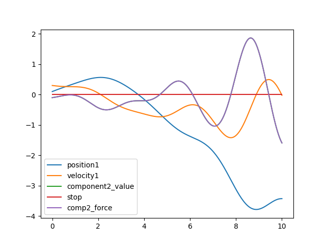
Note that the output dictionary also includes a ‘stop’ flag, which we’ll touch on later.